Simulation & Statistics in R

- INTRODUCTION
- Concept Of Simulation
- Why do we simulate ?
- Drawing of Simple Random Sample
- Example
- Unequal Probability Sampling
- Similating Coin Tosses
- Find the Proportion of heads & tails in long run
- Find the Proportion of heads & tails in long run
- Finding Probabilities
- Drawing a Card
- Divisibility Test
- Urn-Ball Problem
- Urn-Ball Problem
- Birthday Problem
- Card Shiffting
- Cut Shuffle
- Simulating a Cut Shuffle
- Riffle Shuffle
- Simulating Riffle Shuffle
- Simulating Riffle Shuffle
- Simulating Random Variables
- Using it farther
- Much Complicated Ones
- Generating Poisson Distribution
- Continuous Distributions
- Working with inbuilt R functions
- Plotting the normal density
- Other Standard Distributions in R
- Central Limit Theorem
- Law of Laege Numbers
- Plotting the Probability
- Strong Law of large numbers
- Illustrating Strong Law
- Family Planning
- Using Simulation to construct Tests
- Plot of Beta Densities
- What type of test shall we perform ?
- Now lets find the c
- Generating Normal Variables
- Generating Bivariate Normal Variables
- Monte Carlo Simulation
- Bias & Variance
- Monte Carlo Integration
- An assignment Problem
- Brownian Motion
INTRODUCTION
As a statistician, we Want to deal with random experiments. So to do that, thare are various techniques to predict the outcome of such experiments :
Wait and See: Designing winning strategies by trial-and-error method.
Solving Probability Models: Assume a definite mathematical model to predict outcome, sometimes gets complicated.
Simulate Probability Models: Also start with a mathematical model, but instead of computing it mathematically we use computers to perform the virtual random experiment following that model and then analyze the artificial data generated by computers. Similar to “wait and see” except that we do not need to wait long reality.
Concept Of Simulation
Assume a mathematical model.
Use computers to perform the random experiment artificially.
Computers can do artificial random experiment as computers can generate random numbers.
Use the artificial data generated by the computers to analyze the model and predict the outcome.
Note that, the random numbers generated by computers are not random in absolute sense, they are only pseudo-random numbers.
Why do we simulate ?
To have a better understanding of the known probability models.
To visualize a probability model with examples of outcome of a random experiment ( which in reality are hard to obtain )
To have an idea about the result of a statistical model which cannot be solved explicitly using formula.
To judge the performance a model before applying it to a real data situation.
Drawing of Simple Random Sample
- We use the sample() command for both with-replacement & with-out-replacement sampling.
set.seed(123)
sample(c("A","B","C","D","E"),size = 3,replace = F) #-- Without replacement
## [1] "C" "B" "E"set.seed(123)
sample(c("A","B","C","D","E"),size = 3,replace = T) #-- With replacement## [1] "C" "C" "B"Example
set.seed(5)
sample(1:10,size=2,replace = T)
## [1] 2 9set.seed(6)
sample(100,size=5)## [1] 53 10 45 78 56Unequal Probability Sampling
set.seed(7)
sample(c("A","B","C"),size = 2,prob = c(0.1,0.4,0.5))
## [1] "A" "C"Similating Coin Tosses
- An unbiased coin is tossed 10 times. Lets see the output of the tosses.
set.seed(100)
sample(c("H","T"),10,replace = T)
## [1] "T" "H" "T" "T" "H" "H" "T" "T" "T" "H"- Suppose now the probability of head is 2/6
set.seed(100)
sample(c("H","T"),10,replace = T,prob = c(2/6,4/6))
## [1] "T" "T" "T" "T" "T" "T" "H" "T" "T" "T"Find the Proportion of heads & tails in long run
prop=NULL
size1=seq(100,10000,by=1000)
size2=seq(20000,500000,by=10000)
size=c(size1,size2)
for (n in size)
{
  x=sample(0:1,n,rep=T)
  prop=c(prop,sum(x)/n)
}
plot(size,prop,type="l")
abline(0.5,0)
Find the Proportion of heads & tails in long run
##  [1]    100   1100   2100   3100   4100   5100   6100   7100   8100   9100
## [11]  20000  30000  40000  50000  60000  70000  80000  90000 100000 110000
## [21] 120000 130000 140000 150000 160000 170000 180000 190000 200000 210000
## [31] 220000 230000 240000 250000 260000 270000 280000 290000 300000 310000
## [41] 320000 330000 340000 350000 360000 370000 380000 390000 400000 410000
## [51] 420000 430000 440000 450000 460000 470000 480000 490000 500000
## [1] 0.4800000 0.5100000 0.4985714 0.4880645 0.5026829 0.4905882 0.5039344
## [8] 0.5021127 0.5004938 0.5057143 0.4978500 0.5019333 0.5033500 0.5027600
## [15] 0.5003167 0.5004000 0.4984125 0.5031000 0.4990700 0.4997818 0.4995667
## [22] 0.4988692 0.5021143 0.5017067 0.5019000 0.4986529 0.5001111 0.5005684
## [29] 0.5001250 0.4984714 0.4992182 0.4990478 0.4965500 0.4987200 0.4986769
## [36] 0.4991741 0.4989179 0.5002103 0.4991067 0.4998323 0.5003156 0.4998909
## [43] 0.4985824 0.4995286 0.5017111 0.5003432 0.4990737 0.5005205 0.4994575
## [50] 0.4997585 0.4988833 0.4997023 0.5001773 0.5009356 0.5003457 0.5004979
## [57] 0.5000729 0.4997633 0.4996940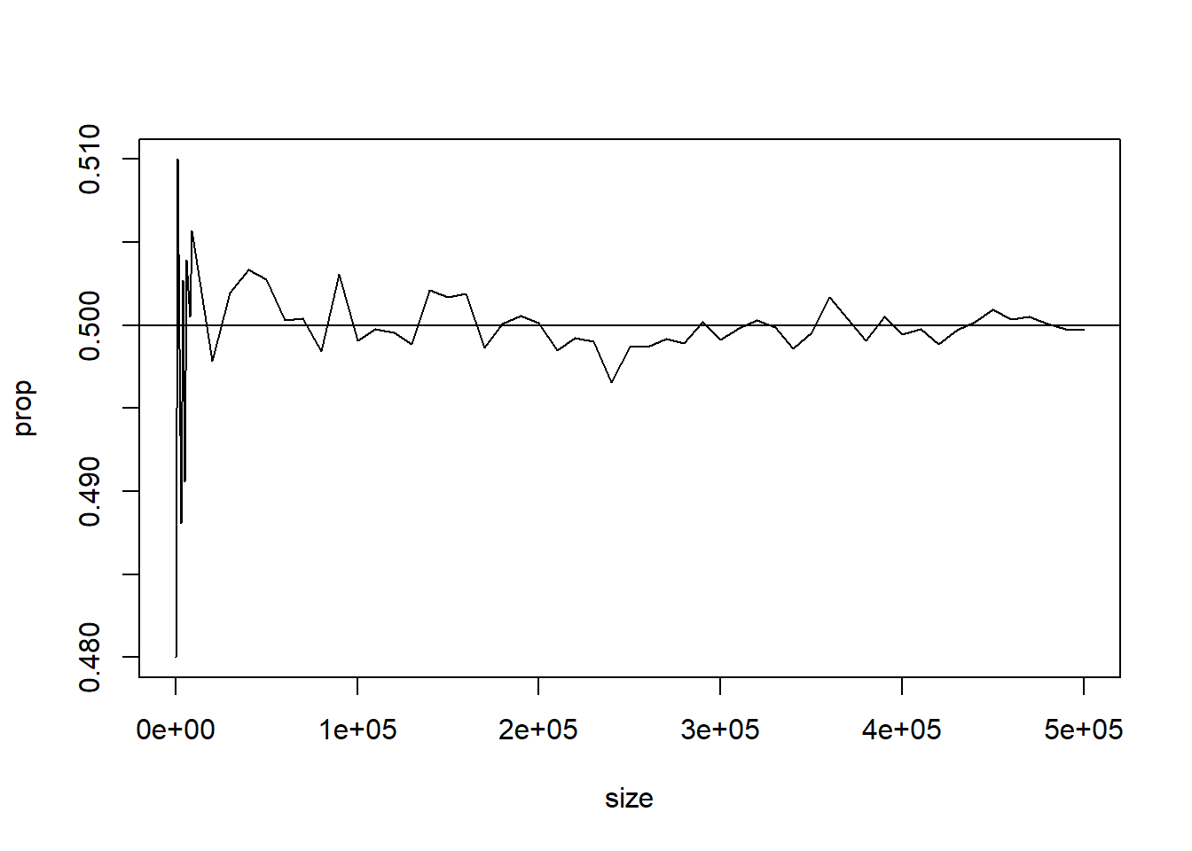
Finding Probabilities
Fact
Probability of any event A can be interpreted as the long term relative frequency of the event A, i.e., \(\frac{no.\;of\;repetitions\;resulting\;in\;A}{total\;number\;of\;repetitions}\) \(as\;n\rightarrow\infty\)
- Hence for computing the probability of any event A by simulation, we shall simulate a large number \(n\) of cases and count the number of times the event A has occurred. If this number is \(m\), then the probability of the event A can be approximated by \(\frac{m}{n}\)
Drawing a Card
- A card is drawn from a full pack of 52 cards. Find the probability that the drawn card is a picture card (i.e., king, queen or jack).
set.seed(125)
pic=NULL
for(i in 1:10000)
{
  x=sample(52,size = 1)
  if(any(x%%13==c(11,12,0)))
  {
    pic[i]=1
  }
  else pic[i]=0
}
sum(pic)/10000
## [1] 0.2287- Because, king= \(11^{th}\) no. card, queen=\(12^{th}\) no. card,jack=\(13^{th}\) no. card.
Divisibility Test
- A number is chosen at random from 1 to 1000. Find the probability that it is divisible by 3, 5 or 6.
count=0
for(i in 1:100000)
{
  num=sample(1000,1)
  if(num%%3==0||num%%5==0||num%%6==0)
  {
    count=count+1
  }
}
count/100000
## [1] 0.46794Urn-Ball Problem
- Suppose an urn contains 7 white and 5 black balls. 3 balls are chosen at random without replacement. Find the probability that :
- all the 3 balls are white
- 2 are white and 1 is black.
Urn-Ball Problem
count1=0; count2=0
balls= as.factor(c(rep("W",7),rep("B",5)))
for ( i in 1:10000)
{
chosen= sample(balls,3)
if (all(chosen=="W")) count1=count1+1
if (table(chosen)["W"]==2) count2=count2+1
}
count1/10000; count2/10000
## [1] 0.1565## [1] 0.4859Birthday Problem
- In a class of 25 students, find the probability that at least two students share the same birthday.
count=0
for(i in 1:500)
{
  ##-- drawing samples by SRSWR --##
  class=sample(365,25,replace = T)
  if(length(unique(class))<length(class))
  {
    count=count+1
  }
}
count/500
## [1] 0.574Card Shiffting
Often we speak of well-shuffled deck of cards.
When we shuffle a deck by hand, the shuffling is always imperfect (not random)
We can simulate these imperfect shuffling in computer.
Cut Shuffle
The simplest method is “cutting” the deck.
We cut the deck at some random point chosen somewhere around the middle of the deck.
Then put the lower part on the top of the upper part.
We shall simulate this shuffle.
Simulating a Cut Shuffle
cut=function(deck)
{
  #choose a random cut point near middle
  x=rbinom(1,52,0.5)
  temp=c(deck[(x+1):52],deck[1:x])
  return(temp)
}
cut(1:52)
## [1] 24 25 26 27 28 29 30 31 32 33 34 35 36 37 38 39 40 41 42 43 44 45 46 47 48
## [26] 49 50 51 52 1 2 3 4 5 6 7 8 9 10 11 12 13 14 15 16 17 18 19 20 21
## [51] 22 23Riffle Shuffle
A much more reliable way is the rifle shuffle ( also known as Faro shuffle or dovetail shuffle)
First split the deck into two parts just as in the cut method.
Take the top half in left hand, and the other half in your right.
Release the cards randomly from both the hands.
Mathematically, if at any stage there are \(a\) cards in your left hand and \(b\) cards in your right, then the next card comes from the left hand with probability \(\frac{a}{a+b}\) and from the right with probability \(\frac{b}{a+b}\).
Simulating Riffle Shuffle
riffle=function(deck)
{
  n=length(deck)
  x=rbinom(1,52,0.5)

  left=deck[1:x]; right=deck[(x+1):52]; k=0;

  a=length(left); b=length(right); tab=NULL;

  for(i in 1:52 )
  {
    ind=rbinom(1,1,a/(a+b))

    if(ind==1)
    {
      tab[k+1]=left[a]

      left=left[1:(a-1)]

      k=k+1; a=a-1
    }
    else
    {
      tab[k+1]=right[b]

      right=right[1:(b-1)]

      k=k+1; b=b-1
    }
  }
  return(tab)
}
Simulating Riffle Shuffle
riffle(1:52)## [1] 26 52 25 51 50 49 48 24 23 22 21 20 47 19 18 46 17 16 45 15 44 43 14 42 41
## [26] 40 39 13 12 11 38 10 9 8 7 37 6 36 35 34 33 5 4 32 3 31 30 2 29 28
## [51] 27 1Simulating Random Variables
We can simulate a Uniform(0,1) variable by the command runif()
This can be used to generate random variables from other discrete and continuous as well.
Suppose we want to generate a Bernoulli random variable with probability of success 0.7
bernoulli=function(prob)
{
  u=runif(1); x=NULL;
  if(u<prob) x=1
  else x=0
  return(x)
}

bernoulli(0.7)
## [1] 0Using it farther
- Suppose we want to simulate a Geometric(0.8) random variable.
x=1
y=bernoulli(0.8)
while(y!=1)
{
  y=bernoulli(0.8)
  x=x+1
}
x
## [1] 1Much Complicated Ones
How can we generate poisson or a Hypergeometric random variable using the above technique ?
For this we need to take the help of the following fact :
Fact
Suppose we want to generate \(X\) having p.m.f. \(P(X=x_i)=p_i\;\;\forall i=0,1,2,...\;\;\sum{p_i}=1\). We generate \(U\sim Uni(0,1)\) and set \[X = \left\{ \begin{array}{rcl} x_0 & if & U<p_0\\ x_1 & if & p_0\leqslant U<{p_0+p_1} \\.&.\\.&.\\x_j & if & \sum^{i-1}_{j=0}p_j\leqslant U<\sum^{i}_{j=0}p_j\\. &.\\. &.\\. &.\end{array}\right.\]
Algorithm
The preceding fact can be written as :
- Generate a random \(U\sim U(0,1)\)
- If \(U<p_0\) stop and set \(X=x_0\)
- If \(U<p_0+p_1\) stop and set \(X=x_1\)
- If \(U<p_0+p_1+p_2\) stop and set \(X=x_2\)
- and so on…
Generating Poisson Distribution
poi_mass=function(x,lambda)
{
  return(exp(-lambda)*(lambda^x)/factorial(x))
}

poi_sample=function(lambda)
{
  U=runif(1); i=0; cumprob=poi_mass(0,lambda)

  while(U>cumprob)
  {
    i=i+1
    cumprob=cumprob+poi_mass(i,lambda)
  }
  return(i)
}
poi_sample(5)
## [1] 2Continuous Distributions
- For continuous distributions we use the following fact :
Fact
(Probability Integral Transformation) If \(X\) has an absolutely continuous distribution, then the C.D.F of \(X\), \(F(x)\) has \(U(0,1)\) distribution.
Suppose we want to generate \(X\) from \(Exp(\lambda)\) distribution.
\[F(x)=1-e^{\lambda x}\;=> U\sim U(0,1)\]
\[X=-\frac{1}{\lambda}ln(1-U)\] is the required random variable.
Working with inbuilt R functions
- Suppose we want to generate random variables from \(N(\mu,{\sigma}^2)\)
# 2 samples from N(5,2) Distribution
rnorm(n=2,mean=5,sd=sqrt(2))
## [1] 7.280889 6.274643- Now let us find \(P(X\leq x)\) i.e., \(\Phi(\frac{x-\mu}{\sigma})\)
# P(X<=4) for N(5,2)

pnorm(4,mean=5,sd=sqrt(2))
## [1] 0.2397501# P(X>7) for N(5,2)
pnorm(7,mean=5,sd=sqrt(2),lower.tail = F)## [1] 0.0786496- We can also compute the normal quantiles \(z_\alpha\)
# lower 0.05 point

qnorm(0.05,mean=5,sd=sqrt(2))
## [1] 2.673826# lower 0.01 point
qnorm(0.01,mean=5,sd=sqrt(2),lower.tail = F)## [1] 8.289953- Can also compute normal density \(\phi(\frac{x-\mu}{\sigma})\)
# density at x=2

dnorm(2,mean = 5,sd=sqrt(2))
## [1] 0.02973257# density at x=5
dnorm(5,mean=5,sd=sqrt(2))## [1] 0.2820948Plotting the normal density
x=seq(-3,3,by=0.01); y=dnorm(x,0,1)
plot(x,y,type="l",main="Density of N(0,1)",ylab=expression(phi(x)))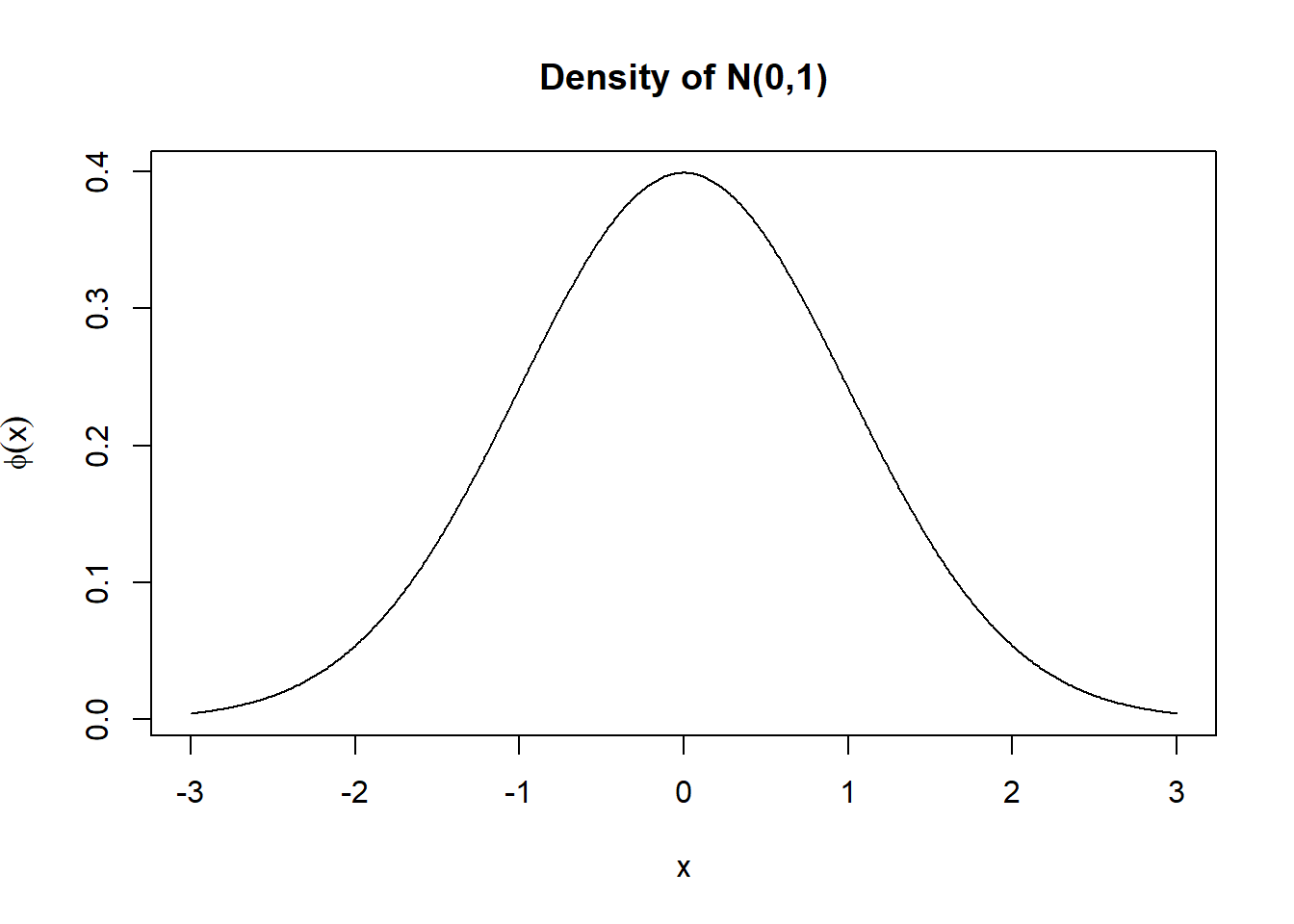
Other Standard Distributions in R
| Distribution | Sample | P(X<=x) | z_alpha | Density |
|---|---|---|---|---|
| Binomial | rbinom(n,size,prob) | pbinom | qbinom | dbinom |
| Poisson | rpois(n,lambda) | ppois | qpois | dpois |
| Neg.Binomial | rnbinom(n,size,prob,mu) | pnbinom | qnbinom | dnbinom |
| Geometric | rgeom(n,prob) | pgeom | qgeom | dgeom |
| Hypergeometric | rhyper(nn,m,n,k) | phyper | qhyper | dhyper |
| Uniform | runif(n,min=0,max=1) | punif | qunif | dunif |
| Exponential | rexp(n,rate=1) | pexp | qexp | dexp |
| Cauchy | rcauchy(n,location=0,scale=1) | pcauchy | qcauchy | dcauchy |
| t | rt(n,df,ncp) | pt | qt | dt |
| F | rf(n,df1,df2,ncp) | pf | qf | df |
| Chi-Square | rchisq(n,df,ncp=0) | pchisq | qchisq | dchisq |
| Gamma | rgamma(n,shape,rate,schale) | pgamma | qgamma | dgamma |
| Beta | rbeta(n,shape1,shape2,ncp) | pbeta | qbeta | dbeta |
| Multinommial | rmultinom(n,size,prob) | - | - | dmultinom |
| Mult.Normal | rmnnorm(n,mean,sigma) | - | - | dmvnorm |
Central Limit Theorem
Theorem
(iid case) Let \(X_1,X_2,...,X_n\) be iid random variables with mean \(\mu\) and variance \({\sigma}^2<\infty\) and \[S_n=X_1+X_2+...+X_n\]. Then, \(\frac{S_n-E(S_n)}{\sqrt{Var(S_n)}}\longrightarrow N(0,1)\) as \(n\longrightarrow \infty\).
\(U_1,U_2,...,U_n\) are iid \(U(0,1)\) variables. Then \[Z_n=\frac{U_1+U_2+...+U_n-\frac{n}{2}}{\sqrt{\frac{n}{12}}}\longrightarrow N(0,1)\;\;;\;as\;\;n\longrightarrow \infty\]
n=100
k=10000
U=runif(n*k)
M=matrix(U,n,k)
X=apply(M,2,sum)
Z=(X-n/2)/sqrt(n/12)
par(mfrow=c(1,2))
hist(Z)
qqnorm(Z)
qqline(Z,col="red")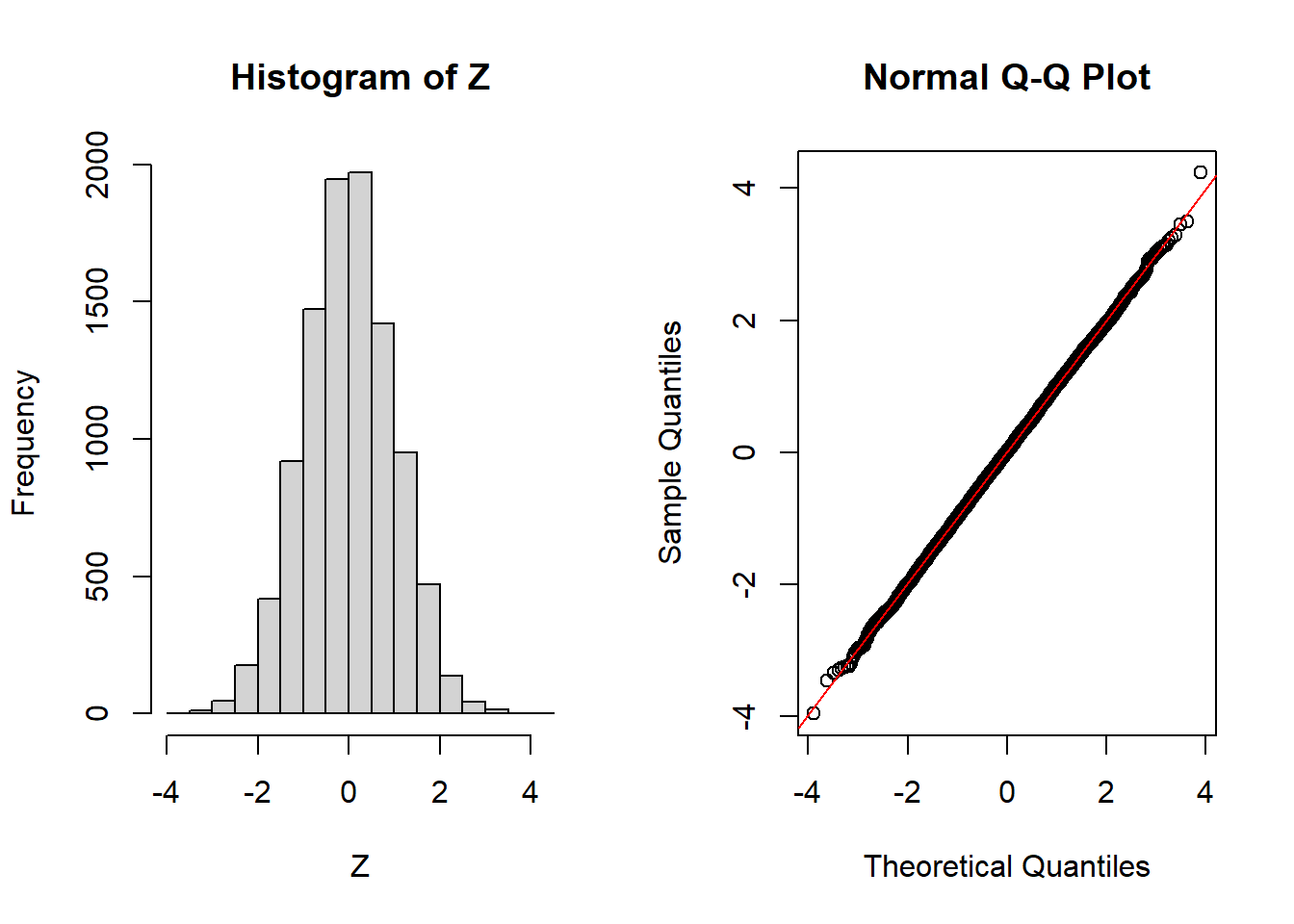
Law of Laege Numbers
The weak Law of large numbers says that for any \(\epsilon>0\) the sequence of probabilities \[P({|\frac{S_n}{n}-\mu|<\epsilon})\longrightarrow 1\;\;\;\;\;as \;\;n\longrightarrow \infty\]
Consider i.i.d. coin flips, that is, Bernoulli trials with \(p=\mu=\frac{1}2\)
We find the \(P({|\frac{S_n}{n}-\mu|<\epsilon})\) in R and illustrate the limiting behavior, with \(\epsilon=0.01\)
Plotting the Probability
wlln=function(n,eps,p)
{
  pbinom(n*p+n*eps,n,p)-pbinom(n*p-n*eps,n,p)
}
prob=NULL
for(n in 1:10000)
{
  prob[n]=wlln(n,eps=0.01,p=0.5)
}
plot(prob,type="l",xlab="n",ylab=expression(P(X<=x)))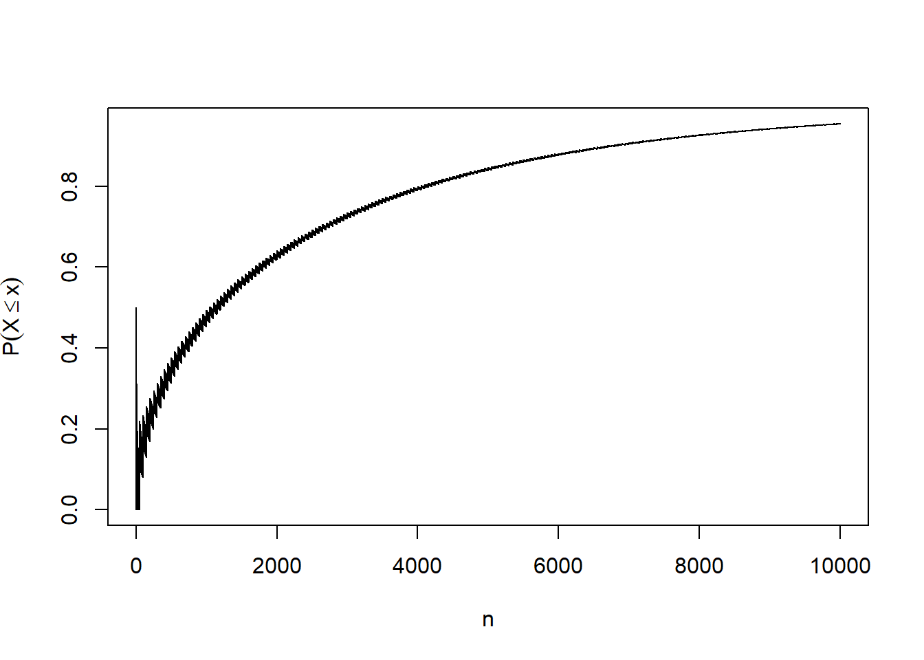
Strong Law of large numbers
The strong law of large numbers says that \(\frac{S_n}n \longrightarrow \mu\;\;\;w.p.\;1\;;\;as\;\;n\longrightarrow \infty\)
Consider i.i.d. coin flips, that is, Bernoulli trials with \(p=\mu=\frac{1}2\)
The sum \(S_n\) is a Binomial random variable.
Illustrating Strong Law
slln=function(n,p)
{
  x=rbinom(1,size=n,prob=p)
  return(x)
}
value=NULL
for(i in 1:10000)
{
  value[i]=slln(i,0.5)/i
}
plot(value,type="l",xlab="n",ylab="Sample mean")
abline(h=0.5)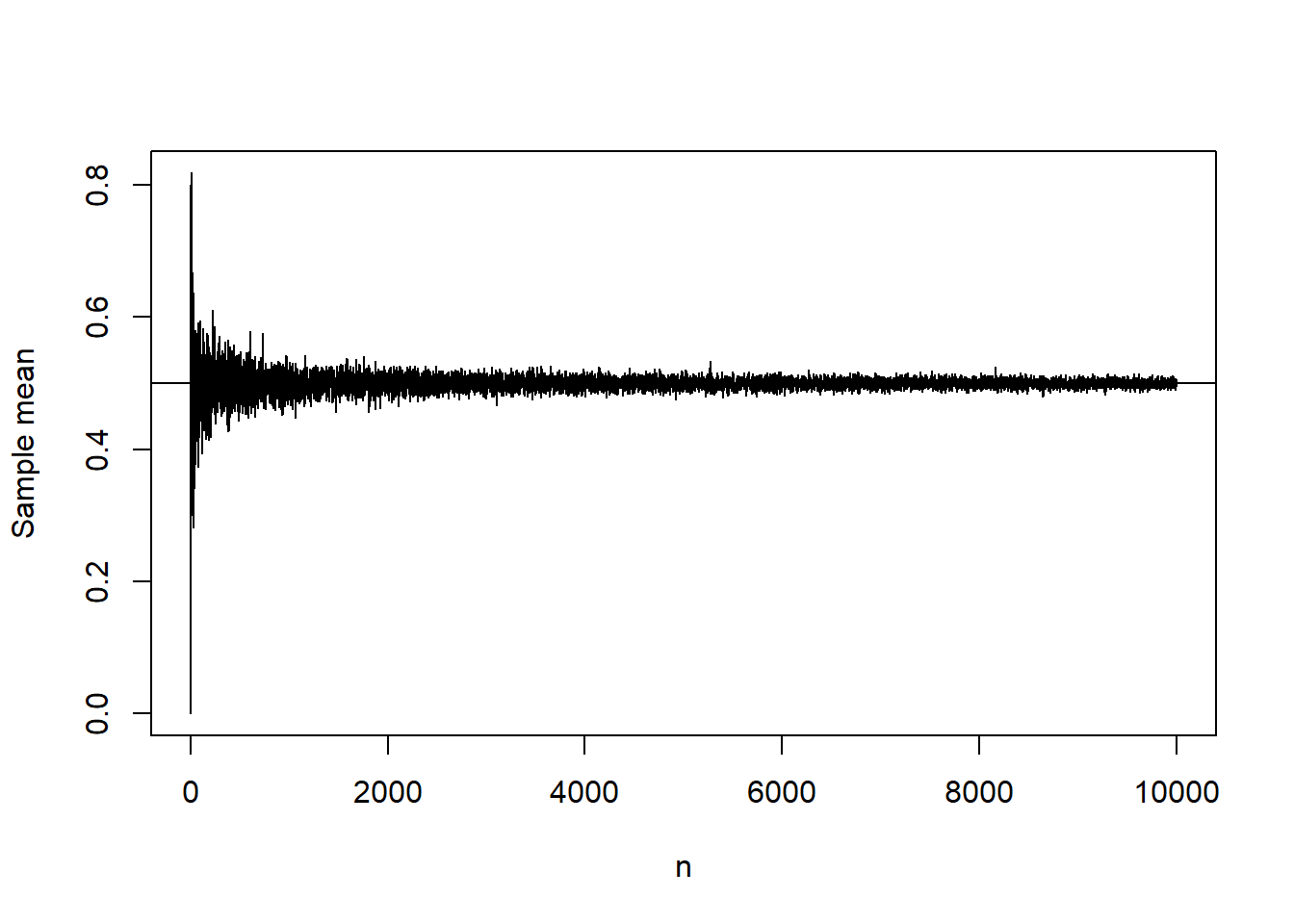
Family Planning
- Suppose a couple is planning to have children until they have one child of each sex. Assuming male and female child are equally probable, how may children can they expect to have ?
count=NULL
for(i in 1:1000)
{
  child=sample(c(0,1),1)
  while(length(unique(child))<2)
  {
    child=c(child,sample(c(0,1),1))
  }
  count[i]=length(child)
}
mean(count)
## [1] 3.08Using Simulation to construct Tests
Simulation can be used to construct tests in situations where the exact sampling distribution of the test statistic is hard to find even under the null hypothesis.
More specially we use simulation to find the \(\alpha100\)% cut-off points
Suppose we have a sample of 101 from Beta(5,b)
We want to test \(H_0:b=5\) against \(H_1:b<5\)
To get an idea about the nature of the test we plot the density function for different values of b.
Plot of Beta Densities
par(mfrow=c(1,3))
x=seq(0,1,by=0.01)
y1=dbeta(x,shape1 = 5,shape2 = 2)
y2=dbeta(x,shape1 = 5,shape2 = 5)
y3=dbeta(x,shape1 = 5,shape2 = 10)
plot(x,y1,type="l",xlab="b<5")
abline(v=median(rbeta(101,shape1 = 5,shape2 = 2)),col="red")
plot(x,y2,type="l",xlab="b=5")
abline(v=median(rbeta(101,shape1=5,shape2=5)),col="red")
plot(x,y3,type="l",xlab="b>5")
abline(v=median(rbeta(101,shape1=5,shape2=10)),col="red")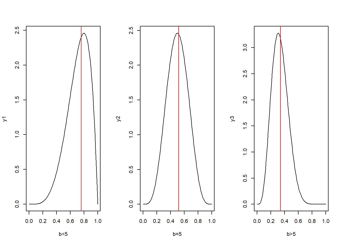
What type of test shall we perform ?
From the figures we see that sample median can be used as a test statistic.
Also a right tailed test based on the median will be appropriate
Thus we shall reject \(H_0\) if the sample median exceeds some value \(c\).
We want to find the test at 90% level of signficance.
We shall use simulation technique to find the cut-off point \(c\).
set.seed(100);prob=NULL; j=1
C=seq(0.2,0.9,by=0.001)
for ( c in C)
{
prob[j]=0
for(i in 1:100)
{
x=rbeta(101,shape1=5,shape2=5)
me=median(x)
if(me>c) prob[j]=prob[j]+1
}
prob[j]=prob[j]/100
j=j+1
}
plot(C,prob,type="l")
abline(h=0.9,col="red")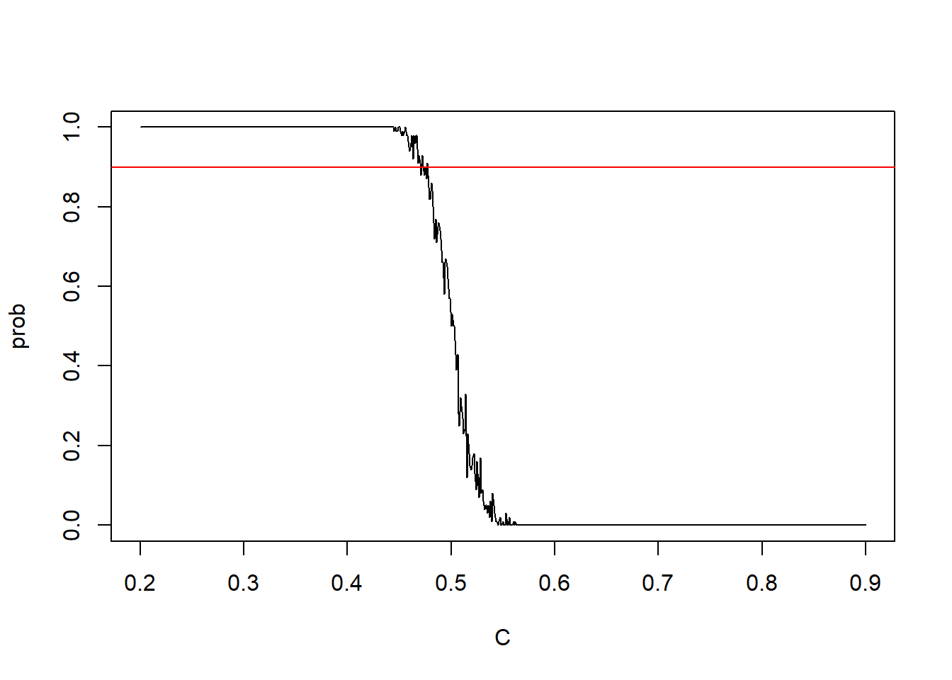
Now lets find the c
We continue to search the c for which \(P_{H_0}(me>c)\) is closet to 0.9
C[which(prob>0.89 & prob<0.91)]## [1] 0.473 0.475prob[which(C %in% C[which(prob>0.89 & prob<0.91)])]## [1] 0.9 0.9So, we can take c to be 0.473 Thus our test rule is: Reject \(H_0\) if sample median exceeds 0.473
Generating Normal Variables
- Instead of using R inbuilt function, rnorm(), we can generate Normal variables from scratch.
Fact: Box-Muller transformation
let, \(U_1\),\(U_2\)\(\sim U(0,1)\)
\[Z_1=\sqrt{-2 ln U_1} cos(2\pi U_2)\] \[Z_2=\sqrt{-2 ln U_1} sin(2\pi U_2)\]
Then, \(Z_1,Z_2 \sim N(0,1)\) independently.
So, to generate \(Y \sim N(\mu , {\sigma}^2)\); we use, \(Y=\mu +\sigma Z\) where, \(Z \sim N(0,1)\).
normal=function(n)
{
  U1 = runif(n)
  U2 = runif(n)
  C = sqrt(-2*log(U1))
  Z1 = C*cos(2*pi*U2)
  Z2 = C*sin(2*pi*U2)
  return(Z1)
}

n = 100000
Z = normal(n)

hist(Z,prob=T,col=rainbow(12))

#-- note that, rainbow() is a graphical function, which gives multiple color.
curve(dnorm(x),-3,3,
      add=T,lwd=4)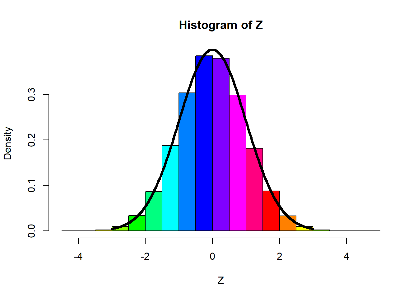
Generating Bivariate Normal Variables
Fact:
If \((X,Y) \sim N_2(0,0,1,1,\rho)\), then \(Z_1=X\) and \(Z_2=\frac{(Y-\rho X)}{\sqrt{1-{\rho}^2}}\) are iid \(N(0,1)\), where, \(-1<\rho<1\)
Equivalently, if we generate \(Z_1\),\(Z_2\) iid \(N(0,1)\), then setting \(X=Z_1\) and \(Y=(1-{\rho}^2)Z_2+\rho Z_1\) gives a pair of random variables that have \(N_2(0,0,1,1,\rho)\) distribution.
binorm=function(n,rho)
{
  x = numeric(n); y<- numeric(n)
  for (i in 1:n)
  {
    z1 = normal(1)
    z2 = normal(1)
    x[i] = z1
    y[i] = rho*z1+sqrt(1-rho^2)*z2
  }
  return(cbind(x,y))
}
n = 1000 ;rho = -0.5

data = binorm(n,rho)

##-- Plotting Bivariate Normal Data --##

plot(data,
     pch=19,
     xlab="X",
     ylab = "Y")

abline(lm(data[,2]~data[,1]),col="red",
       v=mean(data[,1]),
       h=mean(data[,2]),
       lwd=3)

legend("topright",legend = c(paste("mean(X)= ",round(mean(data[,1]),3)),
                              paste("Var(X)= ",round((sd(data[,1]))^2,3)),
                              paste("mean(Y)= ",round(mean(data[,2]),3)),
                              paste("Var(Y)= ",round((sd(data[,2]))^2,3)),
                              paste("samp corr.= ",round(cor.test(data[,1],data[,2])$estimate,2))),
       cex=0.66)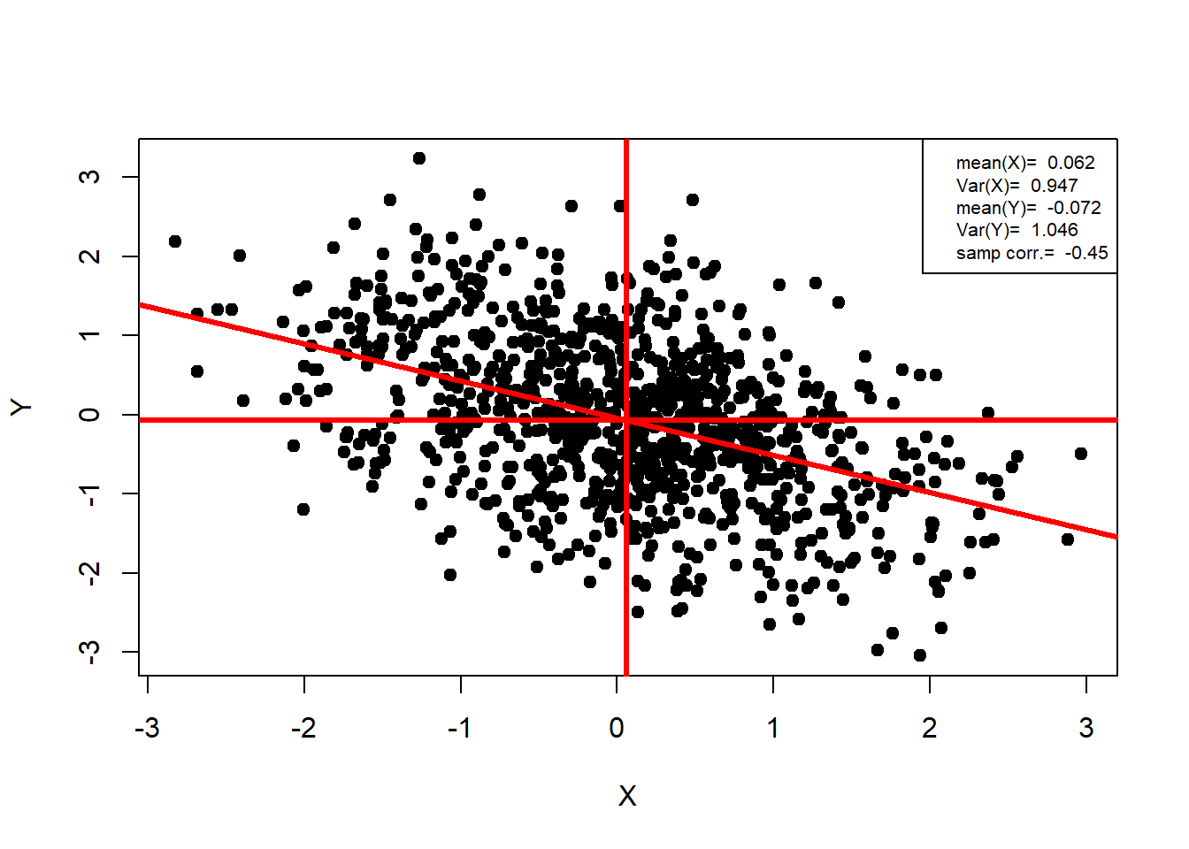
Monte Carlo Simulation
We know that sample average \(\bar{x}\) converges to population mean by consistency property.
Thus expected value of any function can be approximated by the sample average.
Thus \(\frac{1}{N} \sum_{i=1}^N{f(X_i)} \longrightarrow E(f(X))\) with probability 1 as \(N \longrightarrow \infty\) if \(X_1,X_2,...\) are iid sequence of random variables with the same distribution as \(X\).
A Monte Carlo method for estimating \(E(f(X))\) is a numerical method based on the approximation \[Z_N^{MC}=E[f(X)]\approx \frac{1}{N} \sum_{i=1}^N(f(X_1))\] where \(X_1,X_2,...\) are iid sequence of random variables with same distribution as \(X\).
Bias & Variance
- The Monte Carlo estimate \(Z_N^{MC}\) for \(E(f(X))\), has \[bias(Z_N^{MC})=0\] and \[MSE(Z_N^{MC})=Var(Z_N^{MC})=\frac{1}{N} Var(f(X))\]
Monte Carlo Integration
Consider the integral \({\int}_a^bf(x)dx\)
Objective is to approximate this integral
Let \(X_1,X_2,...\) be iid \(U(a,b)\), i.e., density of \(X_j\) is \(\phi(x)=\frac{1}{b-a}I_{[a,b]}\)
Then \[{\int}_a^bf(x)dx=(b-a){\int}_a^bf(x) \phi(x)dx=(b-a)E(f(X))\approx \frac{b-a}{N} \sum_{i=1}^N{f(X_j)}\] for large \(N\)
Example
Evaluate the integral \({\int}_0^{2\pi} e^{k\:cos(x)}dx\)
We, grnerate samples \(X_j\) from \(U(0,2\pi)\)
Then use the approximation \[{\int}_0^{2\pi} e^{k\:cos(x)}dx \approx \frac{2\pi}{N} \sum_{j=1}{e^{k\:cox(X_j)}}\]
set.seed(123)
N = 1000
x = runif(N,min=0,max=(2*pi))
value = sum(exp(cos(x)))
value = (2*pi)*value/N
value
## [1] 7.901431Another Example
Problem: Generate the c.d.f of \(N(0,1)\) for several values of the argument and then compare its accuracy.
The normal c.d.f can be expressed as, \[\Phi(t)= {\int}_{-\infty}^t \frac{1}{\sqrt{2\pi}}e^{\frac{x^2}{2}}dx\]
We shall use Monte Carlo method to estimate \(\phi(t)\) as, \[\phi{(t)} \approx \frac{1}{n} \sum_{i=1}^n{I(X_i \le t)}\] where, \(I(X_i \le t)=\) 1 or 0 with prob. \(\phi(t)\) or \(1-\phi(t)\) respectively, and \(X_i\)’s are random samples from \(N(0,1)\).
n = 1000
t = seq(-3,3,0.01)
x = NULL
phi.hat=NULL
phi=NULL
for(i in 1:length(t))
{
 x = rnorm(n)
 s = sum(x<=t[i])
 phi.hat[i] = s/n
 phi[i] = pnorm(t[i])
}
par(mfrow = c(1,2))
plot(t,phi,main="Original c.d.f",col="red",pch=19)
plot(t,phi.hat,main="Estimated c.d.f",col="blue",pch=19)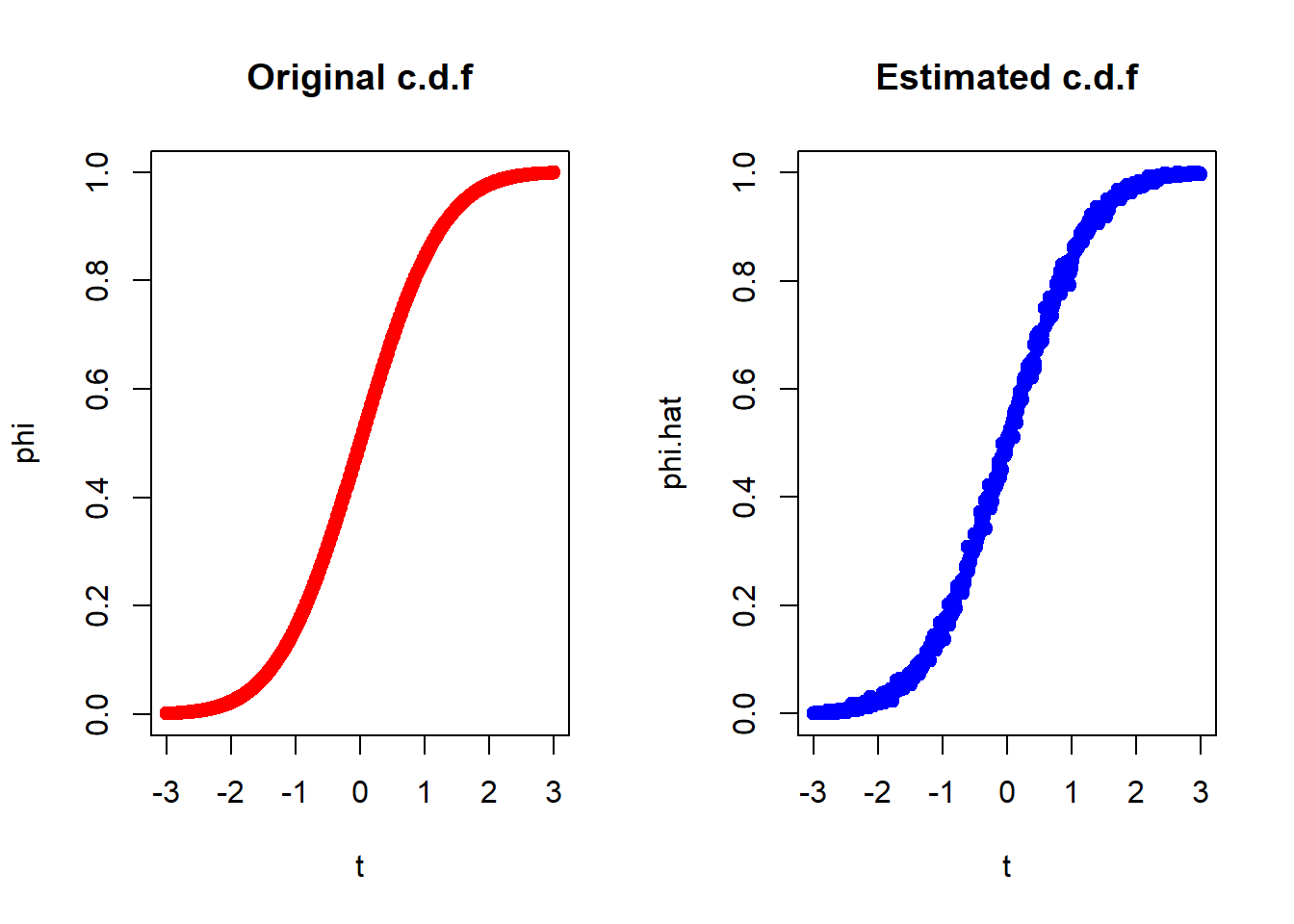
An assignment Problem
Here, we have to do :
Draw a random sample of size 50 from \(N(1,2)\)
Draw another radom sample of size 1000 from the same distribution \(N(1,2)\)
Calculate the test statistic :\(T_n=\frac{\sqrt{n}(\bar{X_n}-1)}{s_n}\)
Repeat this 1000 times.
Draw histograms of the \(T_n\)’s coming from two different samples of the same population \(N(0,1)\)
Copare these two histograms with the Standard Normal distribution.
Solution:
- here, to plot histograms, instead of using the famous ggplot2 package, I am using the basic R plotting function.
##--- Creating a Function to simulate 1000 test statistics for two different samples

simulation=function(len_1,len_2){

  A=NULL
  B=NULL

  for(i in 1:1000)
  {
    Sam_1=rnorm(len_1,1,sqrt(2))
    Sam_2=rnorm(len_2,1,sqrt(2))

    Tn_1=(sqrt(length(Sam_1))*((sum(Sam_1)/length(Sam_1))-1))/sqrt(var(Sam_1))

    Tn_2=(sqrt(length(Sam_2))*((sum(Sam_2)/length(Sam_2))-1))/sqrt(var(Sam_2))

    A=c(A,Tn_1)

    B=c(B,Tn_2)

  }
  Mat=as.data.frame(matrix(c(A,B),ncol=2,byrow = F))
  names(Mat)=c("Tn_1","Tn_2")
  return(Mat)
}

X=(simulation(50,1000)) # Data Table

X[1:10,] # Showing 1st 10 samples of the Data Table
## Tn_1 Tn_2
## 1 0.8020946 0.20259551
## 2 -0.8509208 -1.40945355
## 3 -0.2805664 -1.05684656
## 4 -0.6615001 -0.44404425
## 5 2.3164142 -0.09538437
## 6 -2.3255364 -0.42208845
## 7 -0.2363790 0.60943958
## 8 -2.8176113 -0.40001562
## 9 -0.2177217 -2.25709292
## 10 -0.0575885 2.26107062# Writing a message
writeLines(paste(c("Omitting","the","rest","990","values")),sep=" ")## Omitting the rest 990 values##--- Histogram of the 1st Sample
hist(X$Tn_1,
col="red",
xlab="Tn",
ylab="Frequency",
main="For the Sample 1",
density = 50)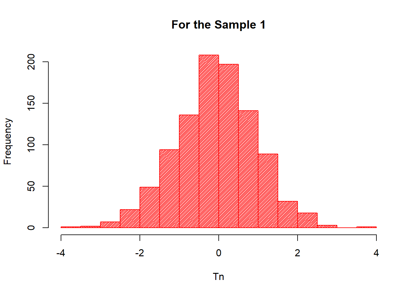
##--- Histogram of the 2nd Sample

hist(X$Tn_2,
     col=12,
     xlab="Tn",
     ylab="",
     main="For the Sample 2",
     density = 40)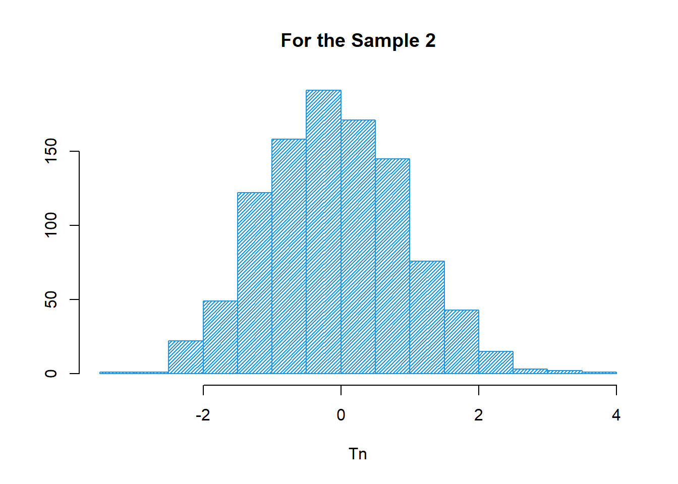
##--- Preparing the density of the N(0,1)

a=seq(-3,3,by= 0.01) # Range of the sample points for N(0,1)

b=dnorm(a) # density of the N(0,1) for the above range.

##--- Comparing Plots :

hist(X$Tn_1,           # histogram for the Sample 1
     col="red",
      xlab="Tn",
      ylab="Frequency",
      main="Comparing Two Histograms coming from two\n different Samples of the same \nPopulation N(1,2) with the Standard Normal density",
     density = 50,
     axes=F,
     cex=4)
par(new=T)             # For Overlap the new plot
hist(X$Tn_2,
      col=12,
      xlab="",
      ylab="",         # histogram for the Sample 2
      main="",
     density = 40,
     axes = F)
par(new=T)             # For Overlap the new plot
plot(a,b,
     type ="l",
     xlab="",
     ylab="",          # Density curve of the N(0,1)
     main = "",
     axes = F,
     col="darkgreen",
     lwd=3)

# Adding Legend

legend("topright",
       legend = c("Sample 1","Sample 2","PDF-N(0,1)"),
       fil=c("red",20,"darkgreen"),
       cex=0.6)

# Adding box

box()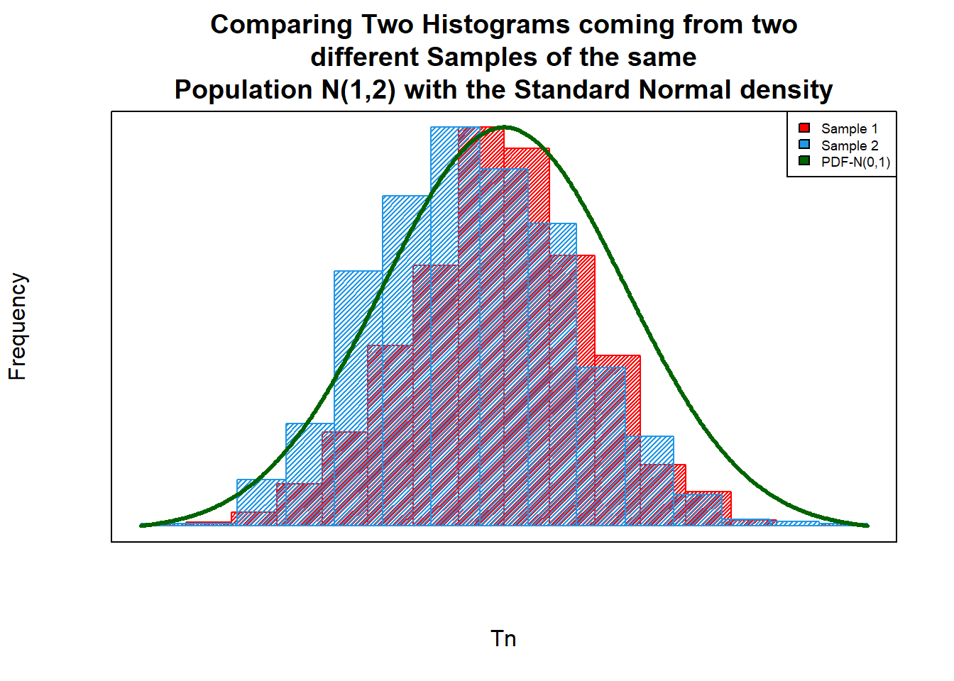
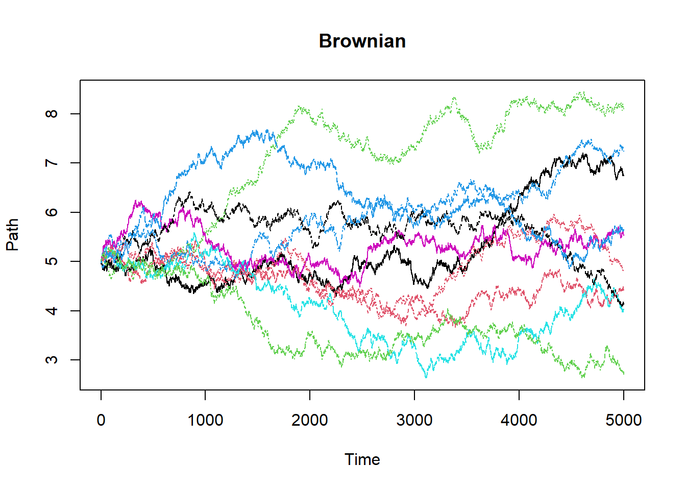
Brownian Motion
Note that the concepts on basics of Monte Carlo Simulation and various Random Distributions have been introduced lets focus on using Monte Carlo methods to simulate paths for various Stochastic Processes.
Standard Brownian Motion on \([0,T]\) is a Stochastic Process \((W(t),0\leq t \leq T)\) which satisfies some properties such as
- \(W(0) = 0\)
- For any \(k\) and any \(0 \leq t_1 \leq .... \leq T\), the increments between any two successive \(W(t_i)-W(t_{i-1})\) are independent.
- The difference \(W(t)-W(s) \sim N(0,t-s)\) for any \(0\leq s<t \leq T\)
As a consequence of 1st and 2nd, \(W(t) \sim N(0,t)\).
On the other hand, Brownian Motion which is non-standard will have two parameters just like Normal Distribution known as drift and diffusion. Using \(W(t)\) we therefore give a Stochastic Differential Equation for any Brownian Motion
\[Brownian\:motion\:with\:drift\: \mu \:and\:\:diffusion\:\:coefficient\: \sigma^2\:\:through\:\:the\;SDE\] \[dX(t)=\mu(t)dt+\sigma(t)dW(t)\]
Sample Paths Generations
Solving the SDE presented above we can write the equation in terms of \(X(t_i),\mu(s),\sigma(s)\) \[X(t_{i+1})=X(t_i)+\int_{t_i}^{t_{i+1}}\mu(s)ds+\sqrt{\int_{t_i}^{t_{i+1}}{\sigma^2(u)du Z_{i+1}}}\] Hence let us look at the code to generate paths where I have assumed \(\mu\) and \(\sigma\) to be constant.
Brownian = function() # This is a function to generate Browninan with drift 0.04 and diffusion 0.7
{
    paths = 10
    count = 5000
    interval = 5/count
    sample = matrix(0,nrow=(count+1),ncol=paths)
    for(i in 1:paths)
    {
        sample[1,i] = 5
        for(j in 2:(count+1))
        {
            sample[j,i] = sample[j-1,i]+interval*0.04+((interval)^.5)*rnorm(1,0,1)*0.7
        }
    }
    cat("E[W(2)] = ",mean(sample[2001,]),"\n")
    cat("E[W(5)] = ",mean(sample[5001,]),"\n")
    matplot(sample,main="Brownian",xlab="Time",ylab="Path",type="l")
}

StandardBrownian = function() # This is a function to generate Standard Browninan with drift 0 and diffusion 1
{
    paths = 10
    count = 5000
    interval = 5/count
    sample = matrix(0,nrow=(count+1),ncol=paths)
    for(i in 1:paths)
    {
        sample[1,i] = 0
        for(j in 2:(count+1))
        {
            sample[j,i] = sample[j-1,i]+((interval)^.5)*rnorm(1)
        }
    }
    cat("E[W(2)] = ",mean(sample[2001,]),"\n")
    cat("E[W(5)] = ",mean(sample[5001,]),"\n")
    matplot(sample,main="Standard Brownian",xlab="Time",ylab="Path",type="l")
}
StandardBrownian()
## E[W(2)] = -0.2205643
## E[W(5)] = -0.2023842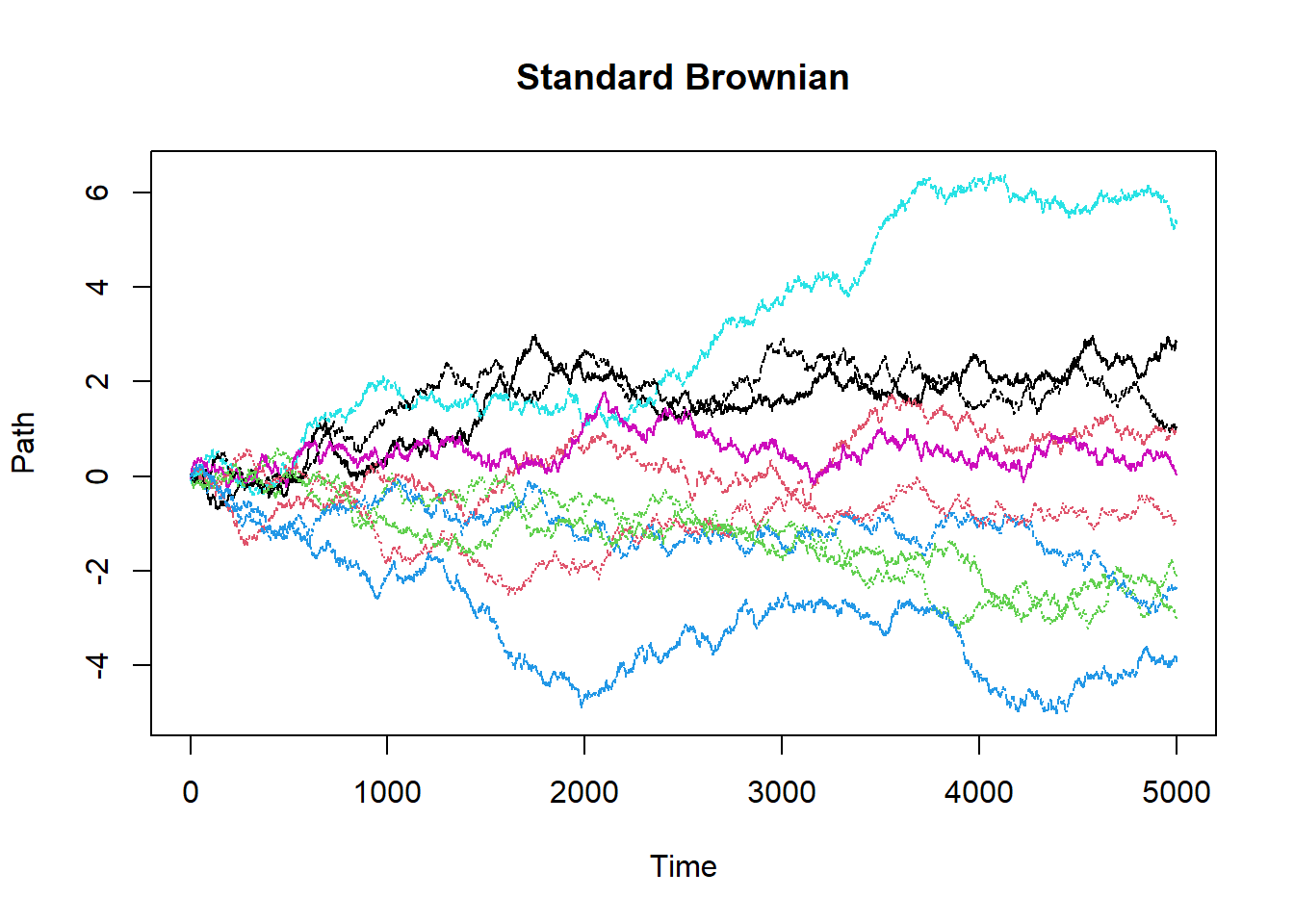
Brownian()## E[W(2)] = 5.321014
## E[W(5)] = 5.338038