Write a user-defined function in R

- INTRODUCTION
- User Defined Functions
- Doing more than one computation
- Default argument of a function
- Additional Arguments
- Data types of arguments
- Sanity checking argument
- Scope of variables
- Recursive Function
- Loops in R
- While loop
- If & If-Else
- If-Else function
- Else if Ladder
- Switch Statement
- Repeat Loop
- Plotting Functions
- Plotting normal curve
- sin(1/x) plot
- Zoom at the origin
- Solving Equation
- Solving Equation
- Solving Equation
- Some Calculus in R
- Optimization
- Further reading
INTRODUCTION
In this tutorial, we will learn, how to make our own custom function in R.Though, R has thousands of functions under thousands of packages, but it is most important to know about how to make a customized function function.
User Defined Functions
Functions are created using the function() directive and are stored as R objects just like anything else. In particular, they are R objects of class function”.
The basic format of the code is
function_name = function(arguments)
{
main computation to be done
}
#---define a function
testfunction = function(x,y)
{
  x+y
}

#--- call the function with arguments 2,5
testfunction(2,5)
## [1] 7Doing more than one computation
- When a function performs more than one task and gives multiple objects return() is used to get all the outputs in a form of a vector.
testfunction = function(x,y)
{
  sum= x+y
  prod= x*y
  return(c(Sum=sum,Product=prod))
}
testfunction(2,5)
## Sum Product
## 7 10- Note that the two output can be accepted separatedly as
result = testfunction(2,5)
result[1]
## Sum
## 7result[2]## Product
## 10- Alternatively multiple output can be extracted using list(). This will enable us to extract by names (along with indices)
testfunction = function(x,y)
{
  sum= x+y
  prod= x*y
  output=list(Sum=sum,Product=prod)
  return(output)
}
output= testfunction(2,5)output$Sum## [1] 7output$Product## [1] 10Default argument of a function
R provides methods to define the default value of the arguments while defining the function.
This default values will be used when the function is called unless this argument values are changed during calling.
#--- initializing x=1 & y=1

testfunction = function(x=1,y=1)
{
  sum= x+y
  prod= x*y

  #--- Creates the output list

  output=list(Sum=sum,Product=prod)
  return(output)
}
testfunction() #-- calling function with no arguments
## $Sum
## [1] 2
##
## $Product
## [1] 1Additional Arguments
- Provision for additional arguments (probably optional arguments, which cannot be decided beforehand) can be done using “…”
testfunction = function(x=1,y=1,...)
{
  sum= x+y
  prod= x*y

  #--- Creates the output list

  output=list(Sum=sum,Product=prod)
  return(output)
}
testfunction(2,5,z=12) #-- z is an extra argument which has no use in this function
## $Sum
## [1] 7
##
## $Product
## [1] 10Data types of arguments
- Since the types of arguments are not specified (at the time of definition), the arguments can be of any type of any data type provided the internal code of the function is conformable with that data type
testfunction = function(x=1,y=1,...)
{
  sum= x+y
  prod= x*y

  #--- Creates the output list

  output=list(Sum=sum,Product=prod)
  return(output)
}
testfunction(2,5,z=12) #-- calling with vectors
## $Sum
## [1] 7
##
## $Product
## [1] 10#-- calling with characters
testfunction("F","M")\(\color{red}{\text{Error in x+y : non-numeric argument to binary operator}}\)
Sanity checking argument
So how can we stop a function if the user calls it with non-conformable arguments ?
A good practice is to write functions in such that while calling, it checks whether the arguments supplied make sense before going to the main body of the function.
testfunction = function(x=1,y=1,...)
{
  #-- check if the arguments are not characters
  stopifnot(typeof(x)!="character",typeof(y)!="character")
  sum= x+y
  prod= x*y

  #--- Creates the output list

  output=list(Sum=sum,Product=prod)
  return(output)
}
testfunction("F","M")
\(\color{red}{\text{Error in testfunction("F","M") : typeof(x) != "character" is not TRUE}}\)
- The stopifnot function halts the execution of the function (with error message) if all of its arguments do not evaluate to TRUE.
Scope of variables
- When we define a variable within a function, it will be local and will not affect any global variable even if the name matches.
f_outer=function()
{
  a=2
  f_inner=function()
  {
    b=5
  }
}
c=10- Then variable c is global to both f_outer and f_inner. For f_inner variable b is local but a is global whereas for f_outer, both a and b are local.
Recursive Function
- R supports recursive function, i.e., a function that calls itself recursively.
#-- Creating a recursive function
fact= function(x)
{
  if(x==0)
  {
    return(1)
  }
  else
  {
    return(x+fact(x-1))
  }
}

fact(5) #-- calling the function with x=5
## [1] 16Loops in R
Loops helps to repeat a job. We first start with for loop.
The syntax is for(variable in sequence) { expression to be evaluated }
Here sequence is an expression which evaluates to a vector(not necessarily in A.P.)
For example all the following are valid for(i in 1:10) for(i in c(2,3,7,9,13,17,19,23)) for(i in c(“A”,“B”,“C”))
The no. of times the expression in loop is evaluated is the length of the sequence.
While loop
The syntax is while(condition) { expression to be evaluated }
The loop repeats its action until the test condition is not satisfied.
Unlike for loop we need not to know in advance how many times the loop will repeat.
If & If-Else
The syntax for if statement is if(condition) { expression }
For a binary situation we can use if-else if(condition) { expression 1 } else { expression 2 }
If-Else function
An alternative better way if-else statements is ifelse() function.
The syntax is new variable= ifelse(Some Condition, Value of new variable if condition is true, value if condition is false)
e.g. category= ifelse(marks>80, “Good”,“Fair”) assigns value Good if marks is more than 80 and otherwise Fair.
The additional advantage is in the condition this function can compare a vector with scalar (interpreted as each element compared to the scalar)
Else if Ladder
- When we have more than two cases we can use else-if ladder
f= function(x)
{
  if(x==1) print(a)
  else if(x==2) print(b)
  else print(c)
}
Switch Statement
An alternative and faster way is switch() statement.
The basic syntax is switch(statement,list)
Here statement is evaluated and based on this value, the corresponding item in the list is returned.
e.g. switch(2,“A”,“B”,“C”) gives the answer “B”. It selects the item no. 2 from the list.
switch(4,“A”,“B”,“C”) gives NULL as there is no item with index 4 in the list.
switch(“color”,“color”=“red”,“shape”=“round”,“length”=5) gives answer red (it matches the string)
stat= function(x,type)
{
  switch(type,"mean"=mean(x),
         "median"=median(x),
         "sd"=sd(x))
} #--- function ends here

stat(1:10,"mean") #-- call the function with mean
## [1] 5.5stat(1:10,"median") #-- call the function with median## [1] 5.5Repeat Loop
- Basic syntax is
repeat { expression to be evaluated }
No default way of termination.
We need to manually terminate the loop using break statement.
x=1 #-- Take any value x as 1
repeat
{     #-- Loop begin here
  x=x+1
  if(x==6) break #-- manual instruction to exit loop
}   #-- Loop ends here

x #-- checking the value of x
## [1] 6Plotting Functions
Any function can be plotted using curve()
The syntax is curve(function,from,to,n,add=T/F,…) where from and to are range over which the function is plotted and n(integer) is the number of points at which we evaluate. add=TRUE/FALSE indicates whether to add this curve to a existing plot or not.
To get more information about it’s arguments type ??curve()
  myfun= function(x)
  {
    x*(1-x)
  }
  curve(myfun,from=0,to=1)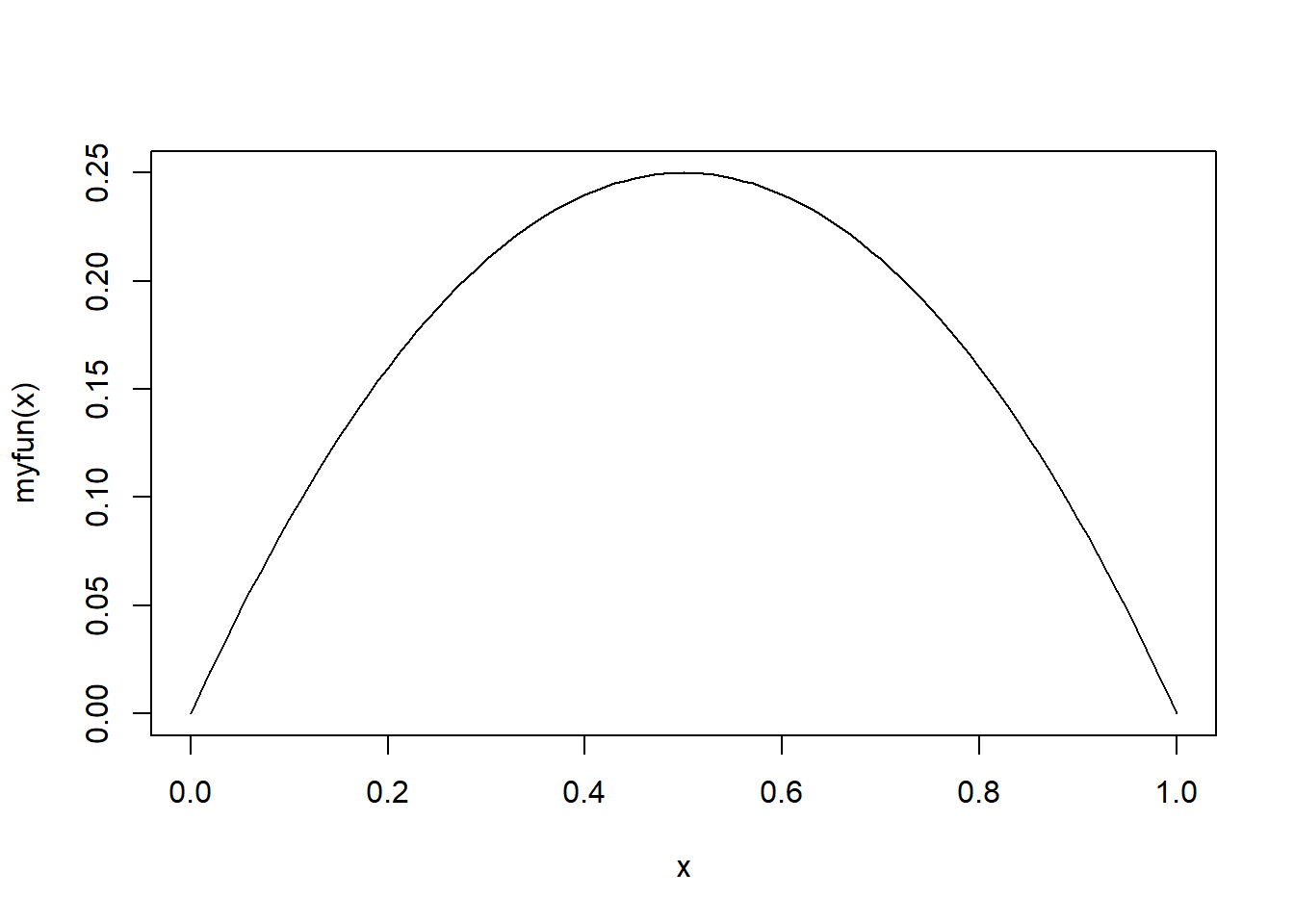
Plotting normal curve
  #-- dnorm gives pdf of N(0,1)
  curve(dnorm,from = -4,to=4,n=500)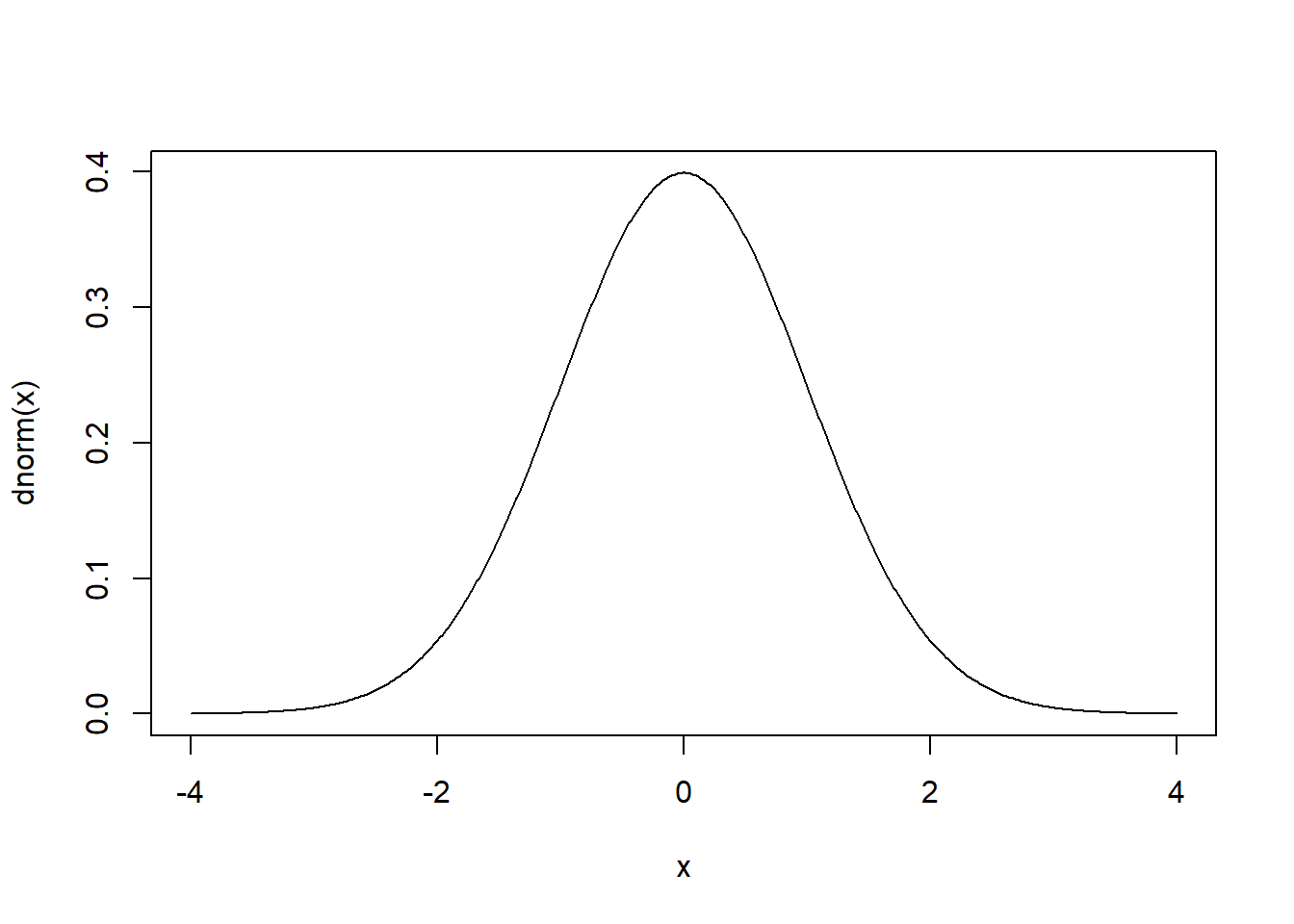
sin(1/x) plot
curve(sin(1/x),from = -2,to = 2)## Warning in sin(1/x): NaNs produced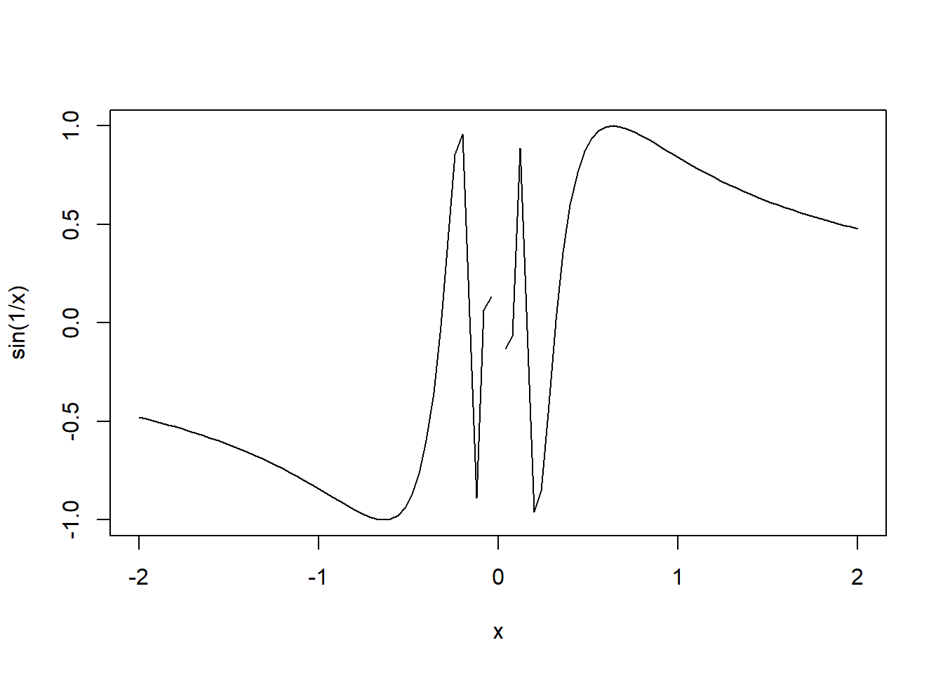
Zoom at the origin
curve(sin(1/x),from = -0.1,to = 0.1)## Warning in sin(1/x): NaNs produced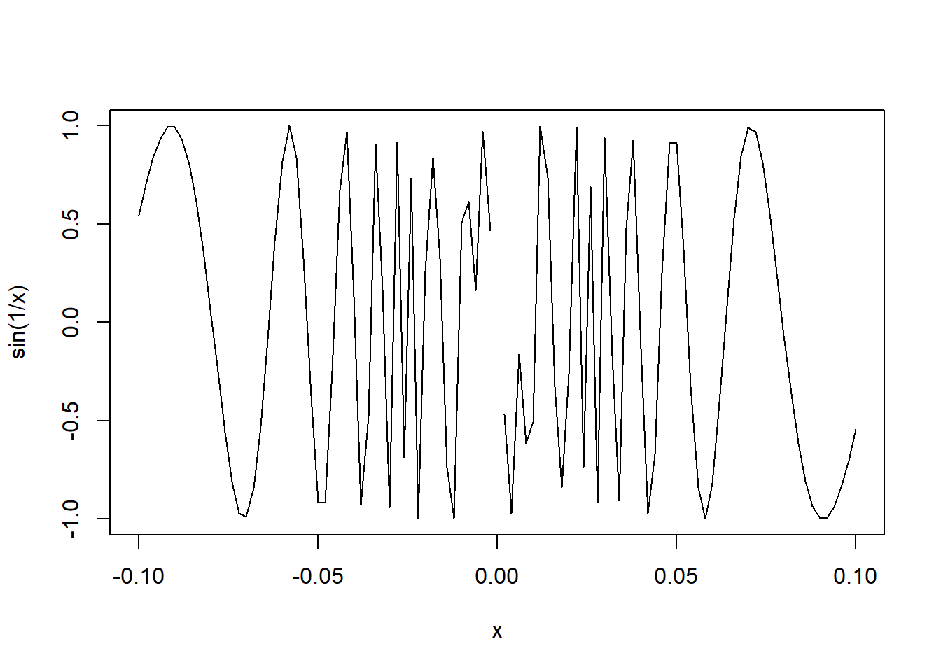
Solving Equation
Already we know if we have a system of equations we can use solve()
For equations involving one variable we can use uniroot()
The syntax is uniroot(function,interval,…)
For solve \[e^x=sin(x)\] we write
uniroot(function(x) exp(x)-sin(x),c(-5,5))Solving Equation
## $root
## [1] -3.183063
##
## $f.root
## [1] -1.359327e-08
##
## $iter
## [1] 8
##
## $init.it
## [1] NA
##
## $estim.prec
## [1] 6.103516e-05
Solving Equation
For finding real or complex roots of a ploynomial use polyroot()
For solving roots of \(n\) non-linear equations we can use multiroot() from the rootSolve package.
Some Calculus in R
Define integral can be done using integrate()
e.g. \(\int_0^1(x^2)dx\) can be done using
integrate(function(x) x^2,0,1)## 0.3333333 with absolute error < 3.7e-15- For derivatives, we use deriv()
Optimization
Maximum or Minimum value of a function can be found using optimize()
optimize(function,interval,maximum=TRUE/FALSE)
optimise(function(x) exp(-x),c(0,5))## $minimum
## [1] 4.999936
##
## $objective
## [1] 0.006738379- There are other functions for optimization like optim(),nlm(),constrOptim().